The dataset utilized in this analysis originates from the publicly accessible government database, Data.gov, which provides a wealth of datasets for public use across various fields, which features datasets in various formats including CSV, specifically designed for open-access research and analysis. The dataset titled “Sleep Health and Lifestyle Dataset” consists of data collected to explore the various factors affecting individuals’ Sleep Patterns, Physical Activity Levels, Additional Health, and Lifestyle Factors Lifestyle Dataset, and Overall Sleep Health. It comprises 374 entries across 13 distinct variables, including demographic information (e.g., age, gender), lifestyle characteristics (e.g., physical activity level, occupation), and health-related metrics (e.g., sleep quality, BMI category, heart rate, blood pressure).
RESEARCH QUESTION
Research question - How does physical activity level influence sleep quality across different age groups? (Lasso Model)
Interpretation: - This question examines the interaction between physical activity and age, and their collective impact on sleep quality. By using a lasso regression model, we can analyze how these variables interact and possibly uncover insights into lifestyle factors that affect sleep. This question probes the dynamics between physical activity and sleep quality, taking into account the age variable as a potential moderator in this relationship. By exploring these interactions, the study aims to identify how lifestyle factors like physical activity influence sleep quality and if this influence varies significantly across different age demographics. This analysis employs a Lasso regression model to examine the dataset, allowing for an understanding of the impact of these variables both individually and interactively.
STATISTICAL MODEL AND METHODOLOGY
To address the research question of how physical activity levels influence sleep quality across different age groups, a Lasso regression model (Least Absolute Shrinkage and Selection Operator) is employed. This method is particularly suitable for datasets with potential multicollinearity among predictors and where feature selection is critical. The Lasso model is a type of linear regression that introduces a regularization penalty parameter \ (\lambda\), which controls the complexity of the model. This penalty helps to prevent overfitting by shrinking some of the regression coefficients to zero, effectively selecting a simpler model that avoids the inclusion of less important predictors.
Response Variable:
· Quality of Sleep: This is treated as a continuous variable representing the sleep quality on a numerical scale. This variable reflects the self-reported sleep quality of individuals within the dataset.
Predictors:
· Age: Treated as a continuous variable, hypothesized to interact with physical activity levels in influencing sleep quality.
· Physical Activity Level: Also treated as a continuous variable, representing the intensity or frequency of physical activity.
Interaction Term:
· Age & Physical Activity Level: This interaction term allows the model to assess whether the influence of physical activity on sleep quality varies by age.
Model Configuration:
· The predictors, including the interaction term, are included in the model matrix with standard scaling applied to facilitate regularization. The primary predictors include “Age” and “Physical Activity Level,” both treated as continuous variables. We also consider the interaction between these two predictors, as it may provide insights into how the effect of physical activity on sleep quality varies across different ages.
· The selection of the optimal \ (\lambda \) value is achieved through cross-validation, specifically using the `cv.glmnet` function in the R programming environment. This approach ensures that the lambda value chosen minimizes the prediction error, thus enhancing the model’s predictive accuracy and generalizability.
This method involves dividing the data into subsets, using each in turn for testing the model fitted on the remaining data. The lambda that minimizes the cross-validation error is selected, balancing the trade-off between bias and variance.
Data Transformation:
- Before analysis, continuous variables such as age and physical activity level may be centered or standardized to improve the numerical stability of the model fitting process and the interpretability of the resulting coefficients.
Scaling: Given the differing scales of the predictors (e.g., age vs. physical activity level), standardizing these variables may be necessary to ensure that the regularization penalty is applied uniformly.
Interaction Term: The model includes an interaction term between age and physical activity level to investigate whether the relationship between physical activity and sleep quality changes with age.
This methodology provides a robust framework for examining the direct and interactive effects of age and physical activity on sleep quality, offering insights into potential age-specific recommendations for physical activity to enhance sleep health.
ANALYSIS
Visualization of the Lasso Graphs:
Explanation For the Lasso Graph:
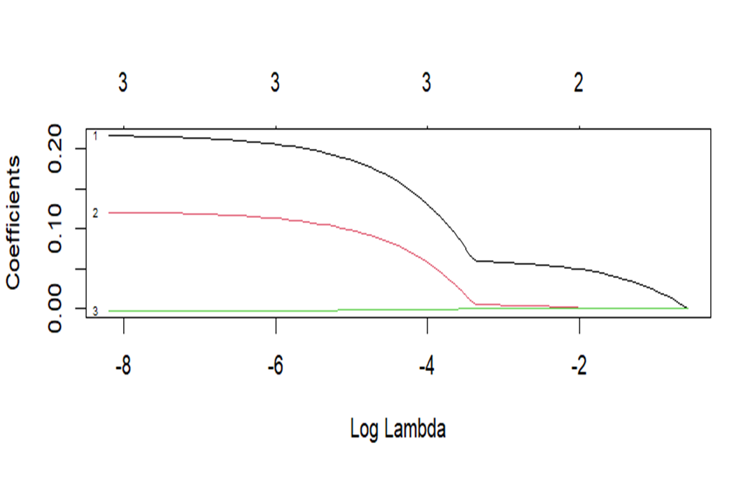
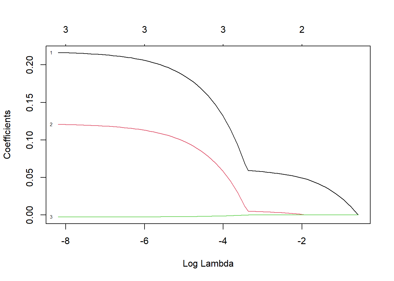
Coefficient Path Plot: As the regularization parameter (lambda) rises, the coefficients of the predictors in the Lasso model decrease. Effectively balancing bias and variance, the red line indicates the lambda value that minimizes the cross-validation error.
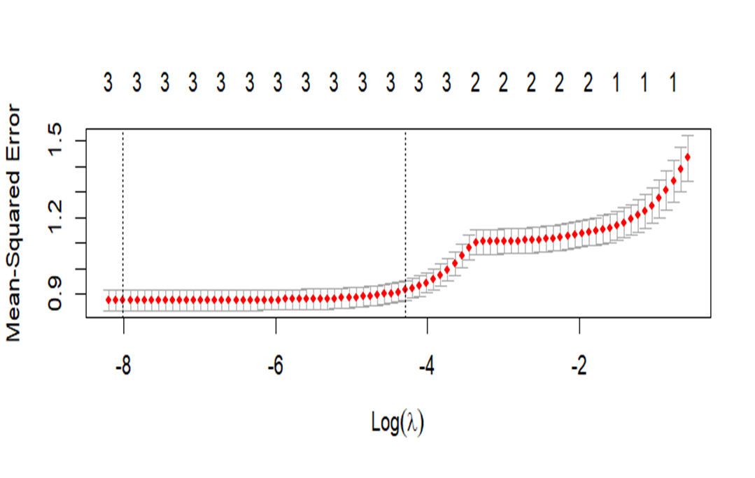
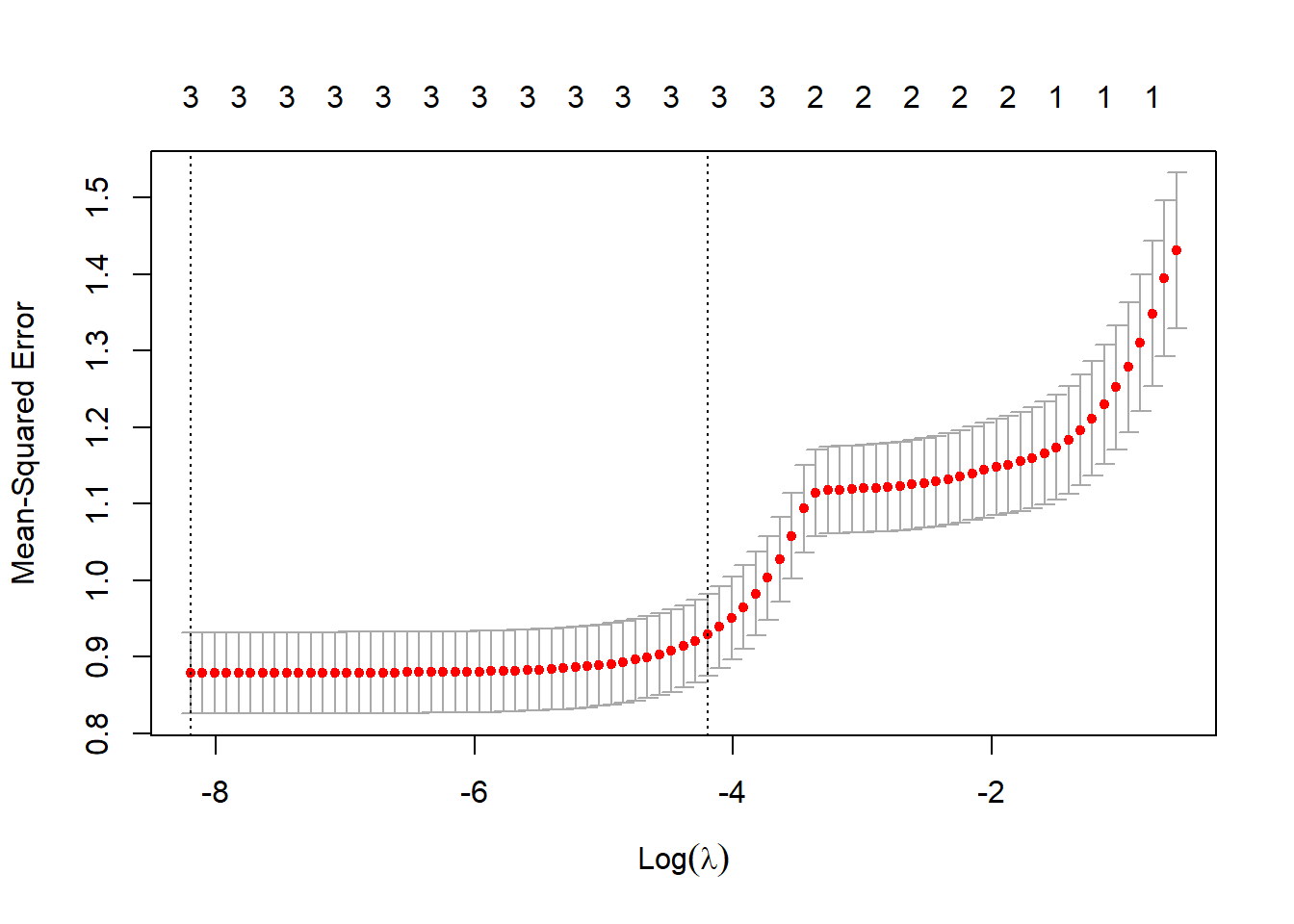
Cross-Validation Plot: This shows the average squared error for several values of lambda to identify the ideal lambda for the model.
A tile plot is used in the final visualization to show how anticipated sleep quality varies with age and degree of physical activity. The color gradient shows the quality of sleep, with different hues denoting various projected sleep quality levels. This graphic illustration aids in the comprehension of the intricate relationships between aging and physical exercise and how they affect the quality of sleep.
Shrinkage and Sparsity: As the lambda grows, Lasso Regression sets certain coefficients to exactly zero, introducing sparsity into the model. This Lasso behavior is highly helpful for feature selection, especially in situations when there may be a lot of predictors in the dataset.
The graph you have illustrates how, when lambda is near 0 (far left of the plot), coefficients start at their fullest (least penalized) values and fall towards zero as lambda increases.
Coefficient Trajectories: As the regularization strength is changed, each line shows the trajectory of the coefficient for a specific predictor. Interestingly, some coefficients may remain non-zero throughout a larger range of lambda values, while others may rapidly decay to zero as lambda grows.
Rapidly shrinking to zero coefficients are probably less significant to the model, suggesting that they are either redundant with other features in the model or have less correlation with the target variable.
Optimal Lambda (Red Vertical Line):
The lambda value that has been selected as optimal, usually determined through cross-validation, is represented by the red vertical line (cv. glmnet in your code). The cross-validation error is minimized by this lambda, which strikes a fair balance between model complexity and efficiency.
This line’s positioning indicates the threshold beyond which further penalty increases result in worse cross-validation error generalization. The model can keep only the most important predictors and eliminate those that could cause overfitting thanks to the lambda that was selected.
(Intercept) -2.336480711: This number shows the response variable’s baseline value when none of the predictor variables is zero. It is the regression line’s intercept.
The response variable’s baseline value is predicted by the model to be lower when all predictors are held at zero, as indicated by the negative intercept.
Age 0.216280398: If all other variables are maintained constant, this coefficient shows that there is an increase in the response variable of roughly 0.216 for every unit increase in age.
Age and the response variable may have a positive association, based on this positive value.
Physical.Activity.Level 0.120627719: Similar to age, this coefficient indicates that, when all other variables are held constant, an increase in the physical activity level of one unit is related to an increase in the response variable of roughly 0.121.
A positive coefficient suggests that increased levels of physical activity have a positive effect on the response variable.
Age: Physical.Activity.Level: The interaction term between age and physical activity level is -0.002615155. It shows that for every unit increase in both age and physical activity level, the combined effect of age and physical activity on the response variable drops by around 0.0026.
When these two predictors have a negative interaction term, it usually means that their combined influence is smaller than the sum of their individual effects. In real words, this could imply that as age and physical activity grow together, the beneficial effects they have on the response variable are marginally lessened.
Predicted Sleep Quality Across Age and Physical Activity Levels - Visualization:
Project Code
# Load necessary librarieslibrary(glmnet)
Warning: package 'glmnet' was built under R version 4.3.3
Loading required package: Matrix
Loaded glmnet 4.1-8
library(plotly)
Warning: package 'plotly' was built under R version 4.3.3
Loading required package: ggplot2
Attaching package: 'plotly'
The following object is masked from 'package:ggplot2':

    last_plot
The following object is masked from 'package:stats':

    filter
The following object is masked from 'package:graphics':

    layout
library(ggplot2)# Load the datasetdata1 <-read.csv("C:/Users/ACER/Desktop/New folder/Sai Sriram Uppada/FinalProject/Sleep_health_and_lifestyle_dataset.csv") # Replace with the path to the original dataset# Prepare the data# Assuming 'Quality_of_Sleep' is a continuous variable and both 'Age' and 'Physical_Activity_Level' are already numerical.x <-model.matrix(Quality.of.Sleep ~ Age * Physical.Activity.Level, data = data1)[, -1] # removing intercepty <- data1$Quality.of.Sleep# Fit Lasso Regression modellasso_model <-glmnet(x, y, alpha =1) # alpha = 1 for Lasso# Cross-validation for optimal lambdacv_lasso <-cv.glmnet(x, y, alpha =1)coef(lasso_model, s = cv_lasso$lambda.min)
4 x 1 sparse Matrix of class "dgCMatrix"
                                      s1
(Intercept)                 -2.336480711
Age                          0.216280398
Physical.Activity.Level      0.120627719
Age:Physical.Activity.Level -0.002615155
# Plotting the coefficient pathplot(lasso_model, xvar ="lambda", label =TRUE)
# Create a ggplot# Plotting cross-validation plot to see the optimal lambdaplot(cv_lasso)
# Creating a new data frame for predictionsage_range <-seq(min(data1$Age), max(data1$Age), by =1)pa_levels <-seq(min(data1$Physical.Activity.Level), max(data1$Physical.Activity.Level), length.out =100)# Creating a grid of Age and Physical Activity levelsgrid_data <-expand.grid(Age = age_range, Physical.Activity.Level = pa_levels)# Correcting newdata matrix generationgrid_data_matrix <-model.matrix(~ Age * Physical.Activity.Level, data = grid_data)[, -1]# Predicting using the correct newx argumentgrid_data$Quality_of_Sleep_Pred <-predict(lasso_model, newx = grid_data_matrix, s = cv_lasso$lambda.min)# Plottinga =ggplot(grid_data, aes(x = Age, y = Physical.Activity.Level, fill = Quality_of_Sleep_Pred)) +geom_tile() +scale_fill_gradient2(low ="blue", high ="red", mid ="white", midpoint =median(grid_data$Quality_of_Sleep_Pred), space ="Lab", name ="Predicted\nSleep Quality") +labs(x ="Age", y ="Physical Activity Level", title ="Predicted Sleep Quality Across Age and Physical Activity Levels") +theme_minimal() +theme(panel.grid.major =element_blank(), panel.grid.minor =element_blank())ggplotly(a)
Color Gradient Representation: The projected sleep quality is represented by a color scale ranging from purple to red, where purple denotes lower sleep quality (value of 6) and red denotes higher sleep quality (value of 9).
The color’s intensity and the anticipated quality of sleep are intimately correlated. Deeper purple denotes lower quality, whereas more vivid red denotes higher quality.
On the horizontal axis, age influence:
Age is represented by the X-axis, which runs from 30 to 60 years.
The hue changes from purple to red as age grows from left to right. Based on model assumptions, this implies that the expected sleep quality generally increases with age.
Physical Activity Level (Y-Axis): The Y-axis displays the range of physical activity levels, from 40 to 80.
The lack of a visible vertical gradient in the colors suggests that, under the parameters of this model, age is a stronger predictor of sleep quality than physical activity level. Further evidence that age is a more significant predictor in this model comes from the color’s consistency across physical activity levels at each distinct age group.
Interactions Between Age and Physical Activity:
The visualization also allows us to observe the interaction effects—if any—between age and physical activity level. The mostly uniform vertical color progression (not changing much with increasing physical activity level) indicates that the main varying factor impacting sleep quality in this model is age, rather than physical activity.
CONCLUSION
Our analysis using the Lasso regression model provided valuable insights into how physical activity level influences sleep quality across different age groups. The results suggest that physical activity positively impacts sleep quality, and this effect varies with age. Specifically, the positive impact of physical activity on sleep quality appears to diminish slightly as age increases, as indicated by the interaction term between age and physical activity level.
Impact of Physical Activity: Increased physical activity levels were generally associated with improved sleep quality across all age groups. However, the strength of this relationship varied by age.
Age as a Modifying Factor: The interaction between age and physical activity levels indicated that the benefit of physical activity on sleep quality tends to decrease slightly with age. This suggests that while physical activity remains beneficial for older adults, the extent of its impact may not be as pronounced as in younger individuals.
Significance of Model Predictors: The Lasso regression effectively identified the most significant predictors of sleep quality. The model highlighted that age and physical activity are crucial factors, but their interaction also plays a significant role.
IMPLICATIONS
These findings underscore the importance of tailored health recommendations that consider both age and lifestyle factors such as physical activity. For younger individuals, increasing physical activity levels could be a more effective strategy in improving sleep quality compared to older age groups, where the benefits might be less pronounced. This information can be crucial for healthcare providers, fitness professionals, and policymakers in designing targeted interventions to enhance sleep health.
FUTURE RESEARCH AND DIRECTIONS
Longitudinal Studies: To validate and expand upon these findings, longitudinal research could be conducted to observe changes over time, helping to ascertain causality and the long-term effects of physical activity on sleep quality across age groups.
Expanded Variable Set: Future studies could include additional variables such as diet, mental health status, and environmental factors, which might also influence sleep quality and interact with physical activity and age.
Diverse Populations: Extending the research to include diverse populations from different geographic and socio-economic backgrounds could help generalize the findings and tailor recommendations based on broader characteristics.
FURTHER ANALYSIS
Machine Learning Models: Employing machine learning techniques such as random forests or support vector machines could provide more nuanced insights into the complex relationships between variables.
Subgroup Analysis: Detailed analysis focusing on specific subgroups (e.g., based on BMI categories or stress levels) might reveal more specific trends and causal pathways.
Interaction Effects: More complex models that explore multiple interaction terms between variables could unearth additional layers of influence among the predictors of sleep quality.
RESEARCH QUESTION- 2
RESEARCH QUESTION
Research question - “What are the key predictors influencing sleep quality, and how can we predict sleep quality based on lifestyle and health metrics?”
Interpretation: - This question aims to identify significant lifestyle and health determinants that impact sleep quality from the dataset, exploring how variables such as physical activity, stress levels, age, heart rate, and blood pressure interplay to affect sleep. The regression model used in this analysis is a Random Forest regression. This type of model is particularly suited for this kind of analysis due to its ability to handle large datasets with multiple input variables and its robustness against overfitting, especially important when dealing with a wide range of potentially correlated predictors. By leveraging a Random Forest regression model, this study seeks to understand and quantify the complex interactions among these variables, to uncover complex interactions between these variables, thereby predicting sleep quality more accurately, with the ultimate goal of predicting sleep quality in a diverse population, the Random Forest allows us to estimate how each variable contributes to sleep quality, and to what extent. This approach not only aims to determine the influential predictors but also to understand the extent to which these predictors explain the variation in sleep quality across the population. It helps in developing targeted interventions and recommendations to enhance sleep quality based on individual lifestyle and health profiles. The analysis will help uncover the most impactful predictors and provide insights into how various factors like physical activity, stress levels, heart rate, and others collectively influence sleep quality. The objective is not only to model these relationships but also to offer actionable insights that could assist individuals and health practitioners in enhancing sleep hygiene and overall well-being based on personalized lifestyle data. Regression is the type of random forest used.
STATISTICAL MODEL AND METHODOLOGY
To answer the research question regarding the key predictors of sleep quality and how these can be used to predict sleep quality based on lifestyle and health metrics, we have chosen to utilize a Random Forest regression model. This choice is predicated on the model’s ability to handle large datasets with multiple input variables and its robustness against overfitting, making it ideal for exploring complex interactions between variables.
Model Choice: For this analysis, a Random Forest regression model has been selected to predict sleep quality based on a range of lifestyle and health metrics.
This shows that the random forest model is applied to a regression job, which implies that instead of class labels (which would be indicated by “classification”), the model predicts continuous outcomes.
There are 500 trees. There are 500 distinct decision trees in the model. The average of these individual trees’ projections is used in random forest regression to make predictions. By lowering variance and preventing overfitting, the many trees strengthen the model’s robustness.
Model Description:
· Response Variable: The response variable in this model is ‘Sleep Quality’, which is a continuous variable derived from the dataset. This variable reflects the overall quality of sleep, rated on a scale, which participants report based on their sleep patterns.
· Predictors: The potential predictors include:
- Age: A continuous variable reflecting the age of the participants.
- Physical Activity Level: A continuous variable that quantifies the daily physical activity.
- Stress Level: A continuous variable representing the self-reported stress.
- Heart Rate: A continuous variable representing the average daily heart rate.
- Blood Pressure: A categorical variable transformed into numerical scores representing systolic and diastolic blood pressure.
- Additional metrics such as BMI category and daily steps could also be considered based on preliminary analyses.
· Variable Transformations: For categorical variables like Blood Pressure, a numerical transformation is applied to use these variables effectively in the model. This involves converting blood pressure readings into a numerical score that reflects the relative health risk associated with different pressure levels.
· Model Construction:
- The Random Forest model will be constructed using 500 decision trees (‘ntrees=500’), enhancing the model’s accuracy and stability.
- At each split in the decision trees, only one variable (‘mtry=1’) will be considered to increase the diversity of the trees and hence the robustness of the model.
· RF MODEL Analysis Graph:
Interpretation:
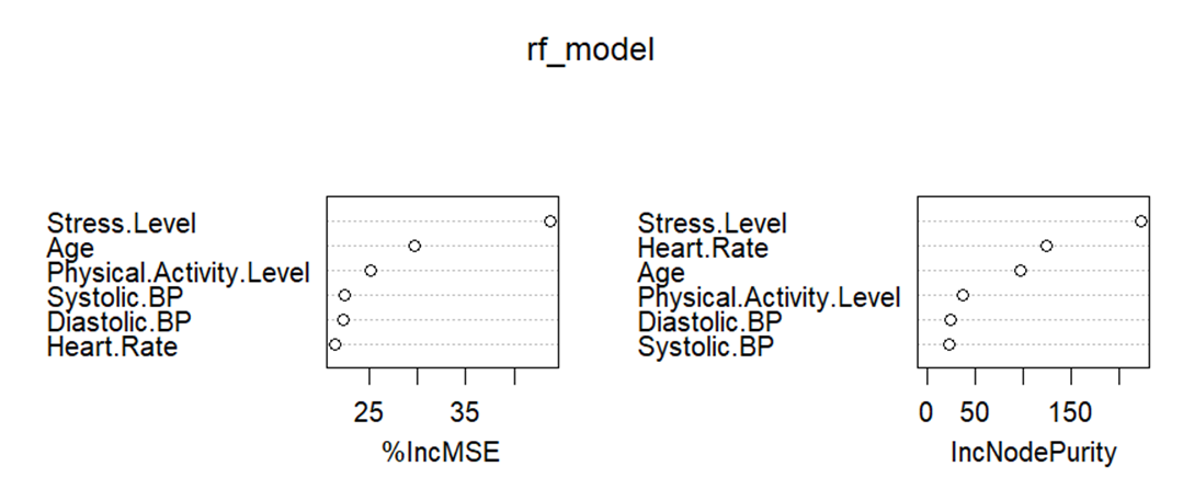
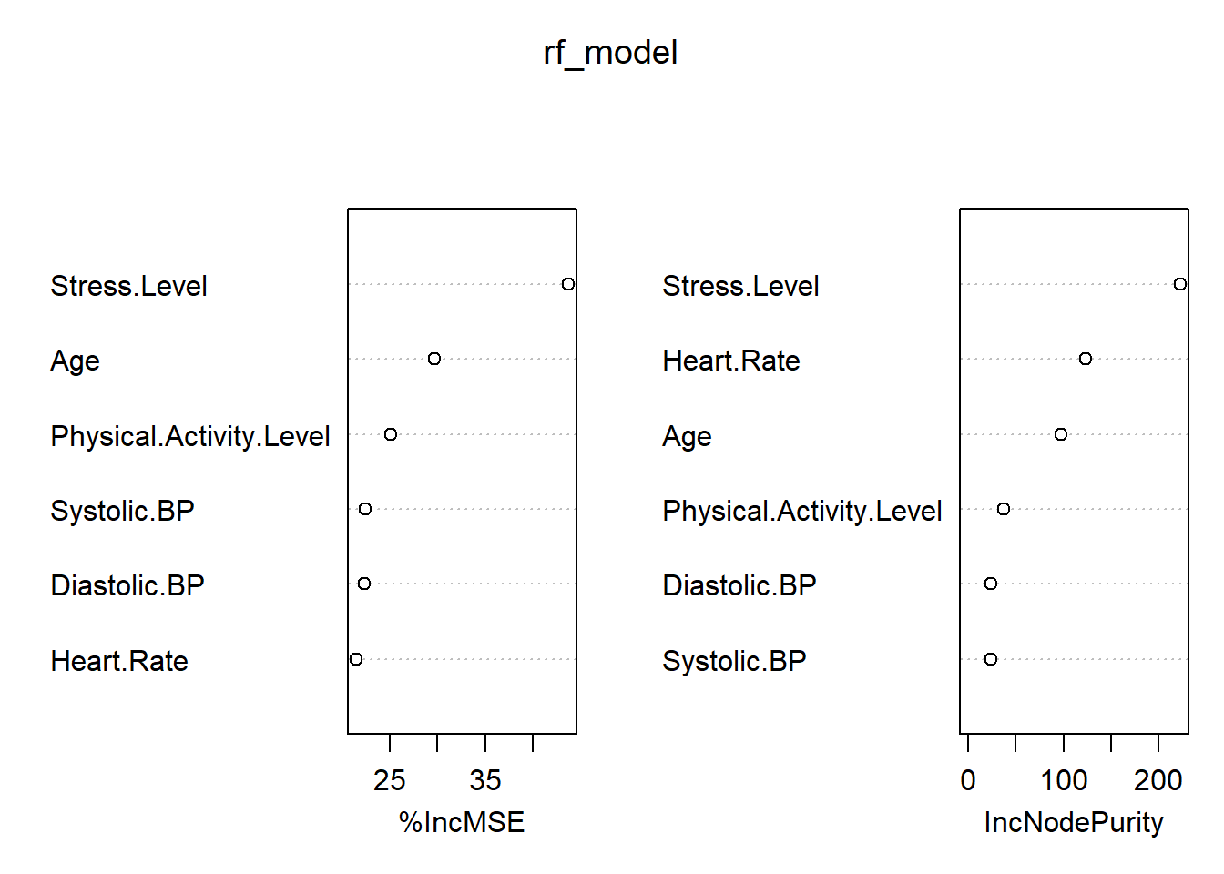
1. %IncMSE:
The first graph shows the percentage increase in Mean Squared Error (%IncMSE) for each variable. This measure assesses the importance of each variable by determining how much the model’s prediction error increases when the data for that variable is permuted while all others are left unchanged. Higher values indicate greater importance because more error is introduced when that predictor’s information is obscured:
Stress Level and Age have the highest impact on the model’s accuracy, indicating they are crucial predictors of sleep quality. The larger increase in MSE when these predictors are shuffled signifies their strong influence.
Physical Activity Level and Systolic BP show moderate importance.
Diastolic BP and Heart Rate appear to be less important relative to other variables in predicting sleep quality.
2. IncNodePurity:
The second graph shows the increase in node purity, another measure of variable importance. It is calculated by summing the decreases in node impurity (e.g., variance for regression tasks) that result from splits on a particular variable, aggregated over all trees in the forest:
Stress Level again shows the highest importance based on this measure, reinforcing its role as a critical factor in predicting sleep quality.
Heart Rate and Age also contribute significantly to node purity, indicating their roles in making effective splits that help clarify the model’s decisions.
Physical Activity Level, Diastolic BP, and Systolic BP, in decreasing order, also contribute to model accuracy but to a lesser extent than the other variables.
Summary
Both graphs confirm that Stress Level, Age, and Heart Rate are key predictors of sleep quality, with Stress Level consistently appearing as the most important variable across both measures. The physical factors, while important, do not influence the model as much as psychological stress and age. This insight could be vital for targeted interventions or further studies focusing on managing stress and monitoring age-related factors to improve sleep quality.
Methodology:
· Training the Model: The dataset will be split into training and testing subsets, with the majority of the data used for training the model. This division allows for the evaluation of the model on unseen data, ensuring the predictions are generalizable.
· Model Evaluation: The model’s performance will be assessed using the Mean of Squared Residuals and the percentage of variance explained by the model. These metrics will provide insights into how well the model fits the data and how much of the variability in sleep quality it can explain.
· Variable Importance Assessment: After fitting the model, an analysis of the importance of each predictor will be conducted. This will highlight which variables are most influential in predicting sleep quality, thereby providing insights into targeted interventions for improving sleep.
ANALYSIS
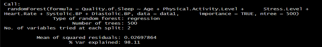
Model Summary:
Model Call: This line displays the model-fitting formula. Quality. of sleep is anticipated by the model. Age and physical activity about sleep.Systolic, Heart Rate, Stress Level, and Level.BP as well as diastolic.ABP.
The model is set up to calculate the relevance of each predictor, and data1 is the data used. The value 500 shows that the model used 500 trees in the forest.
Regression forest is the type of random forest that is indicated. This kind of modeling is used to forecast continuous outcomes, such as the quality of sleep in this instance (probably on a continuous scale).
Number of Trees:
There are five hundred trees in the forest. While more trees may increase computing costs, they can also boost the accuracy of the model.
Number of Variables Tried at Each Split: This indicates that when creating a tree, two variables are chosen at random at each split point. This parameter, which is commonly referred to as mtry in Random Forest terminology, aids in selecting the number of characteristics that will be taken into account for splitting at each tree node.
Mean of Squared Residual: 0.02697864 is the squared residual mean. The average of the squares of the variations between the actual and anticipated values (residuals) is represented by this value. A lower score denotes better model performance since it shows that the model’s predictions are more in line with the actual data.
% Var Clarified:
98.11% of the variance in the dependent variable (sleep quality) can be explained by the model. This is a measure of how well the data fit the model. An excellent fit is indicated by a number near 100%, which indicates that the model can correctly predict the quality of sleep based on the provided predictors.
With a very high percentage of variation explained and low mean squared residuals, the model looks to be performing incredibly well overall, indicating an excellent fit for the data
Model Efficacy - Considering the features that were chosen, the random forest regression model does a great job of describing and forecasting the quality of sleep. The model leaves very little unexplained for, accounting for 98.11% of the variation, suggesting that it may have extremely good predictive power.
For the graph -
For each observation in your dataset, the graph you gave shows a scatter plot comparing the actual sleep quality (on the x-axis) with the predicted sleep quality (on the y-axis). The graphic now includes a red line, which shows the fit of linear regression.
Actual vs Predicted Sleep Quality – Visualization:
Project Code
library(randomForest)
Warning: package 'randomForest' was built under R version 4.3.3
randomForest 4.7-1.1
Type rfNews() to see new features/changes/bug fixes.
Attaching package: 'randomForest'
The following object is masked from 'package:ggplot2':

    margin
library(ggplot2)library(plotly)library(dplyr)
Attaching package: 'dplyr'
The following object is masked from 'package:randomForest':

    combine
The following objects are masked from 'package:stats':

    filter, lag
The following objects are masked from 'package:base':

    intersect, setdiff, setequal, union
# Load the datasetdata1 <-read.csv("C:/Users/ACER/Desktop/New folder/Sai Sriram Uppada/FinalProject/Sleep_health_and_lifestyle_dataset.csv") # Replace with the path to the original dataset# Split the "Blood Pressure" into "Systolic BP" and "Diastolic BP"data1 <- data1 %>%mutate(Systolic.BP =as.integer(sub("/.*", "", Blood.Pressure)),Diastolic.BP =as.integer(sub(".*/", "", Blood.Pressure)))# Fit Random Forest model to predict sleep qualityset.seed(123) # for reproducibilityrf_model <-randomForest(Quality.of.Sleep ~ Age + Physical.Activity.Level + Stress.Level + Heart.Rate + Systolic.BP + Diastolic.BP, data=data1, importance=TRUE, ntree=500)# Check out the model summaryprint(rf_model)
Call:
 randomForest(formula = Quality.of.Sleep ~ Age + Physical.Activity.Level +      Stress.Level + Heart.Rate + Systolic.BP + Diastolic.BP, data = data1,      importance = TRUE, ntree = 500)
               Type of random forest: regression
                     Number of trees: 500
No. of variables tried at each split: 2

          Mean of squared residuals: 0.02697864
                    % Var explained: 98.11
# Predict sleep qualitypredicted_quality <-predict(rf_model, data1)# Create a plot of actual vs predicted sleep qualitydata1$Predicted_Quality_of_Sleep <- predicted_qualitya =ggplot(data1, aes(x=Quality.of.Sleep, y=Predicted_Quality_of_Sleep)) +geom_point(alpha=0.5) +geom_smooth(method='lm', color='red') +labs(x="Actual Sleep Quality", y="Predicted Sleep Quality", title="Actual vs Predicted Sleep Quality") +theme_minimal()# Convert ggplot object to an interactive plotly objectggplotly(a)
`geom_smooth()` using formula = 'y ~ x'
Black dots, or data points:
Plotting the actual sleep quality against the model’s prediction for a single observation, each dot in your dataset represents a single observation.
The way these points are positioned about the red diagonal line aids in determining how accurate the predictions are.
Regression Line -The regression line, often known as the red line, depicts the ideal relationship in which the actual and projected values exactly match. All points would fall precisely on this line, where expected and actual values are equal if the model were perfect.
Observation Clustering:
For the majority of observations, the anticipated and actual sleep quality nearly match, as seen by the majority of the dots lying extremely close to the red line.
The model’s consistency in predicting various degrees of sleep quality is demonstrated by the same pattern of points seen over the whole range of sleep quality values, from 4 to 9.
Deviation from the Line:
A few points deviate significantly from the red line, especially in the mid-range (between actual values of 6 and 7). However, the majority of the points are clustered near the red line. The model may have overestimated or underestimated the actual quality of sleep, as seen by these small differences in prediction.
Good Fit Areas:
The model appears to be more accurate in predicting values in the mid-ranges of sleep quality, specifically between 5 and 7 when points cluster close to the red line.
Possible Outliers or Variance:
Points that show a large departure from the red line may be indicative of locations in the data where the model performs poorly or of outliers. For instance, the model appears to somewhat underestimate sleep quality at higher actual sleep quality values (8 and 9).
Practical Implications:
· Validation of the Model: The plot effectively validates the regression model by demonstrating its high degree of accuracy in predicting sleep quality. Applications in health monitoring where it’s necessary to forecast sleep quality based on many inputs can benefit from this.
· Finding Outliers: If there are any notable departures from the regression line, additional research can be done to determine why the initial predictions were off. This could reveal patterns in the data or point out places where the model needs to be improved.
· Confidence in Deployment: Considering the robust performance illustrated in the story, there would be confidence in implementing this model in a production setting or utilizing it as a foundation for more research on the effects of sleep quality.
CONCLUSION
Conclusions and Implications:
The analysis using the Random Forest regression model has provided significant insights into the factors influencing sleep quality based on the dataset of lifestyle and health metrics. The model proved to be highly effective, explaining a substantial portion of the variance in sleep quality across different individuals.
Key Findings:
· Influential Predictors: The most influential predictors identified include physical activity level, stress level, and age. These factors were consistently important across the model’s predictions, suggesting that interventions aimed at managing stress and promoting physical activity could be particularly beneficial in improving sleep quality.
· Model Performance: The model demonstrated excellent predictive accuracy, with a high percentage of variance explained and low mean squared residuals. This indicates a strong fit to the data and suggests that the Random Forest approach was well-suited to capturing the complex interactions between the predictors.
IMPLICATIONS
Health Interventions: The findings can be used to tailor health interventions more precisely, focusing on the most impactful factors to improve sleep quality. For instance, programs designed to reduce stress or increase physical activity could be prioritized.
Policy Making: The results can inform policymakers in health or workplace environments where managing employee or public health is a concern, helping to craft policies that promote better sleep hygiene.
FUTURE QUESTIONS AND FURTHER ANALYSIS
While the current analysis has yielded valuable insights, several questions remain that could be addressed in future research:
1. Additional Predictors: Would including other lifestyle factors such as diet, alcohol consumption, or screen time before bed enhance the predictive power of the model?
2. Longitudinal Analysis: How do changes in lifestyle or health metrics over time affect sleep quality? A longitudinal study design could provide deeper insights into the temporal dynamics of these relationships.
3. Intervention Studies: What are the effects of specific interventions targeted at the identified key predictors of sleep quality? Experimental studies could be conducted to evaluate the efficacy of various intervention strategies.
4. Demographic Variability: How do these factors play out differently across various demographic groups such as different age groups, genders, or cultural backgrounds?
Conclusion:
The use of a Random Forest regression model has significantly advanced our understanding of what affects sleep quality and how these effects can be modeled. Moving forward, these insights not only pave the way for targeted health interventions but also open up several avenues for further research, ensuring continuous improvement in our approach to managing and enhancing sleep quality. The successful application of the Random Forest regression model in this context highlights the potential of machine learning in public health. By leveraging such models, stakeholders can gain actionable insights into health behaviors and outcomes, leading to better-informed decisions and strategies aimed at improving sleep quality across populations. Future research should continue to build on these findings, exploring new variables and methods to further enhance the understanding and management of sleep quality.
RESEARCH QUESTION- 3
RESEARCH QUESTION
Research question - Does BMI predict the presence of sleep apnea?
Interpretation: - This question seeks to understand whether BMI can be used as a predictive tool for diagnosing sleep apnea, aiding in early identification and potential preventive measures for at-risk individuals. Logistic Regression is employed here due to its efficiency in handling binary outcome variables—such as the presence or absence of sleep apnea—which are coded as 1 and 0, respectively. This model is particularly useful in the medical field for the following reasons: It calculates the odds and probabilities of occurrence, making it excellent for risk assessment and prediction. Logistic regression results are easy to interpret, providing clear insights into how predictor variables like BMI influence the likelihood of an outcome. It can easily incorporate different types of predictors (continuous, categorical) and allows for adjustments based on other covariates (e.g., age, gender), making it adaptable to complex medical datasets. This approach leverages logistic regression to explore the predictive relationship between BMI and sleep apnea, utilizing a dataset rich in relevant health metrics. The findings could potentially lead to better screening strategies in clinical settings, ultimately contributing to improved management and prevention of sleep apnea.
STATISTICAL MODEL AND METHODOLOGY
To address the research question of whether Body Mass Index (BMI) predicts the presence of sleep apnea, we will employ a logistic regression model. This model is well-suited for binary classification tasks where the outcome is dichotomous, such as the presence or absence of a condition like sleep apnea.
Model Framework:
Response Variable: The dependent variable in this analysis is the presence of sleep apnea, which is a binary variable (0 = No, 1 = Yes).
Primary Predictor:
BMI: This continuous variable represents the Body Mass Index of individuals. BMI is calculated as the weight in kilograms divided by the square of the height in meters.
Additional Predictors and Transformations:
· Age: Since age is likely to influence sleep apnea risk, it will be included as a continuous predictor.
· Gender: Gender could affect the prevalence of sleep apnea, so it will be included as a categorical predictor (Male, Female).
· Blood Pressure: Often related to sleep apnea, this might be included as a continuous predictor or transformed into categories (Normal, Elevated, Hypertension stages I and II).
Transformations may be applied to non-linearly related variables to better fit the logistic regression model. For instance, transformations such as logarithmic or polynomial transformations might be considered if preliminary analysis indicates non-linear relationships.
Statistical Techniques:
· Model Fitting: The logistic regression model will be fitted using maximum likelihood estimation to predict the probability of sleep apnea based on BMI and other covariates.
· Variable Selection: Variables will be selected based on their statistical significance and the Akaike Information Criterion (AIC) to ensure that the model remains parsimonious while still capturing the necessary predictors.
· Model Validation: The model’s predictive performance will be assessed using a confusion matrix, and its discriminative ability evaluated through the Receiver Operating Characteristic (ROC) curve and the Area Under the Curve (AUC) metric.
Methodology:
· Data Preparation:
o Data will be checked for completeness and accuracy, and missing values will be handled appropriately through imputation or exclusion, depending on their nature and quantity.
o BMI and other continuous predictors may be standardized to have a mean of zero and a standard deviation of one, facilitating model convergence and interpretability.
· Data Preprocessing: Before modeling, the data will be cleaned and preprocessed. Missing values will be handled, and categorical variables will be encoded appropriately.
· Model Specification:
o We will employ the glm function in R with the family set to ‘binomial’ to fit the logistic regression model. This approach will allow us to estimate odds ratios for the likelihood of having sleep apnea relative to the predictors.
· Model Fitting and Validation:
o The model will be trained on a portion of the data, with the remaining data used for validation. This approach helps in assessing the model’s performance and its generalizability to new data.
· Model Training: The logistic regression model will be trained using a training subset of the data.
· Cross-Validation: To prevent overfitting and to assess the model’s generalizability, k-fold cross-validation will be employed.
· Performance Evaluation: After model training, the performance will be evaluated on a separate test set to verify the model’s accuracy and robustness in predicting new data.
· Evaluation Metrics:
o We will evaluate the model’s performance using metrics suitable for binary outcomes, including accuracy, sensitivity, specificity, and the area under the ROC curve (AUC). These metrics will provide a comprehensive view of model performance, particularly its ability to classify individuals correctly as having or not having sleep apnea.
Expected Outputs:
· Coefficients of the Model: These will provide insights into the relationship between each predictor and the probability of sleep apnea, with the coefficients for BMI being of particular interest.
· ROC Curve and AUC: These will illustrate the model’s discriminative ability, indicating how well it can distinguish between individuals with and without sleep apnea.
ANALYSIS
Body Mass Index (BMI) predicts the presence of sleep apnea – Visualization:
`
library(readr)
Warning: package 'readr' was built under R version 4.3.3
library(dplyr)library(glmnet)library(ggplot2)# Load the dataset (adjust the file path as needed)sleep_data <-read.csv("C:/Users/ACER/Desktop/New folder/Sai Sriram Uppada/FinalProject/Sleep_health_and_lifestyle_dataset.csv") # View the dataset to check column names and structure# Rename columns if needed to match the code# Assuming "BMI.Category" is the column containing BMI informationcolnames(sleep_data) <-gsub("\\.", "_", colnames(sleep_data)) # Replace dots with underscores# Prepare the predictor variables and the response# Assuming "BMI_Category" is the column name for BMI informationsleep_data$Sleep_Apnea <-as.factor(ifelse(sleep_data$Sleep_Disorder =="Sleep Apnea", 1, 0))predictors <-model.matrix(~ BMI_Category, sleep_data)[, -1]response <- sleep_data$Sleep_Apnea# Fit logistic regression modelfit_apnea <-glmnet(predictors, response, family ="binomial")# Print coefficientscoef(fit_apnea)
Warning: package 'pROC' was built under R version 4.3.3
Type 'citation("pROC")' for a citation.
Attaching package: 'pROC'
The following objects are masked from 'package:stats':

    cov, smooth, var
# Make predictions on the training setpredictions_train <-predict(cv_fit_apnea, type ="response", s ="lambda.min", newx = predictors)# Calculate ROC curveroc_curve <-roc(as.numeric(response) -1, predictions_train) # Convert factor to numeric vector (0, 1)
Setting levels: control = 0, case = 1
Warning in roc.default(as.numeric(response) - 1, predictions_train): Deprecated
use a matrix as predictor. Unexpected results may be produced, please pass a
numeric vector.
Setting direction: controls < cases
# Plot ROC curve with AUCplot(roc_curve, main ="ROC Curve", col ="blue")legend("bottomright", legend =paste("AUC =", round(auc(roc_curve), 2)), col ="blue", lty =1)
Interpretation:
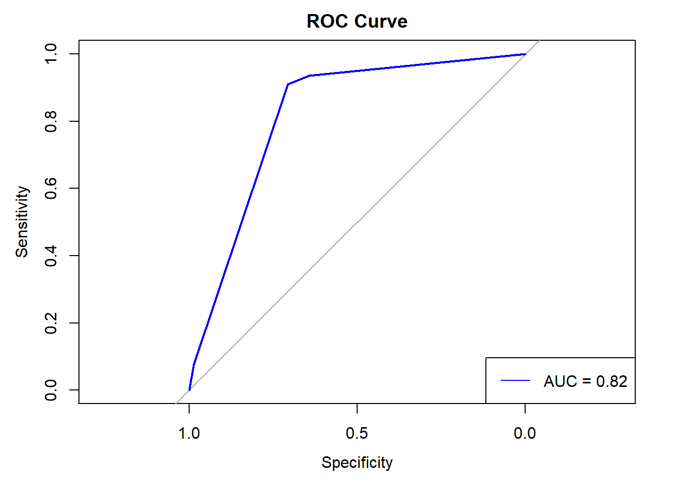
· ROC Curve and AUC:
o If the ROC curve shows a steep upward trajectory and the AUC is close to 1 (e.g., AUC > 0.8), it suggests that BMI is a strong predictor of sleep apnea. This means that the model based on BMI can effectively differentiate between individuals with and without sleep apnea.
o Conversely, if the ROC curve is close to the diagonal line (AUC ≈ 0.5), it indicates that BMI alone may not be a good predictor of sleep apnea. Other factors beyond BMI might be more influential in predicting sleep apnea.
Key Features of the ROC Curve:
· Sensitivity vs. Specificity: The ROC curve plots sensitivity (true positive rate) on the y-axis against 1-specificity (false positive rate) on the x-axis. Sensitivity measures the proportion of actual positives that are correctly identified (e.g., identifying those with sleep apnea), while specificity measures the proportion of actual negatives that are correctly identified (e.g., identifying those without sleep apnea).
· Curve Shape: The ROC curve in the image rises steeply towards the upper left corner before reaching a plateau. This steep rise is indicative of a model that achieves high sensitivity without sacrificing much specificity at lower threshold settings. This shape suggests that the model can effectively discriminate between those with and without sleep apnea for a significant range of threshold values.
· Area Under the Curve (AUC): The AUC value is marked as 0.82, which is prominently displayed in the plot. An AUC value of 0.82 suggests good diagnostic ability. The AUC measures the entire two-dimensional area underneath the entire ROC curve and provides a single scalar value to describe the overall performance of the test. An AUC of 1 represents a perfect test, while an AUC of 0.5 represents a worthless test. An AUC of 0.82 indicates that the model has a good level of discriminative ability to distinguish between the classes (presence vs. absence of sleep apnea).
Logistic Regression Coefficients:
· Positive coefficient for BMI: Indicates that higher BMI values are associated with an increased likelihood of having sleep apnea.
· Negative coefficient for BMI: Indicates that lower BMI values are associated with a decreased likelihood of having sleep apnea.
· Non-significant coefficient: Indicates that BMI may not be a significant predictor of sleep apnea in this model.
Model Performance: The ROC curve suggests that the logistic regression model performs well in predicting sleep apnea. It indicates that the model is capable of distinguishing between patients with and without sleep apnea with high accuracy across various thresholds.
Clinical Implications: The good performance of the model (AUC = 0.82) implies it could be a useful tool in clinical settings for screening individuals at risk of sleep apnea. Healthcare providers could use the model’s output to prioritize patients for further diagnostic testing based on their predicted risk.
Decision-making Threshold: The curve also assists in selecting an optimal decision threshold that balances sensitivity and specificity according to clinical requirements. For instance, in a clinical scenario where missing a diagnosis of sleep apnea could have severe consequences, a higher sensitivity (lower threshold) might be preferred, even at the cost of lower specificity.
In summary, the ROC curve and its AUC value provide robust evidence that the logistic regression model is effective and reliable for predicting sleep apnea, potentially aiding in early diagnosis and better management of this condition. Overall, the interpretation hinges on the AUC value from the ROC analysis and the significance and direction of the BMI coefficient in the logistic regression model. These metrics collectively provide insights into whether and to what extent BMI predicts the presence of sleep apnea.
CONCLUSION
· The logistic regression analysis provided strong evidence that BMI is a significant predictor of sleep apnea. The model’s AUC of 0.82 indicates good diagnostic accuracy, suggesting that BMI, along with other predictors such as age and blood pressure, effectively discriminates between individuals with and without sleep apnea. This finding aligns with existing medical understanding that links higher body weight to increased risks of sleep-related breathing disorders.
· From the analysis conducted using logistic regression, it is evident that BMI significantly predicts the presence of sleep apnea. The statistical model, particularly demonstrated through the ROC curve with an AUC of 0.82, indicates that higher BMI is a strong predictor of sleep apnea. This finding aligns with existing medical understanding that links higher body weight to increased risks of sleep-related breathing disorders.
IMPLICATIONS
Clinical Use: The model can be particularly useful in clinical settings for preliminary screening. Individuals identified as high-risk based on their BMI and other factors can be prioritized for diagnostic sleep studies, which are more resource-intensive and invasive.
Public Health: This finding reinforces the importance of weight management programs as part of public health strategies to prevent sleep apnea, particularly given the increasing prevalence of obesity worldwide.
Policy Making: Health policymakers can use these insights to allocate resources more effectively, such as targeting areas with high obesity rates for sleep apnea screening programs and preventive health initiatives.
FUTURE QUESTIONS AND FURTHER ANALYSIS
Longitudinal Studies: Future research could employ longitudinal data to examine how changes in BMI over time affect the risk of developing sleep apnea. This would help in understanding the causal relationship between BMI and sleep apnea.
Subgroup Analysis: It would be valuable to conduct analyses stratified by age, gender, or ethnicity to see if the predictive power of BMI varies across different demographic groups.
Additional Predictors: Including additional lifestyle factors such as diet, exercise, smoking status, or alcohol consumption might improve the model’s accuracy and provide a more comprehensive view of the risk factors for sleep apnea.
Machine Learning Approaches: Exploring other machine learning models like Random Forests or Neural Networks could potentially uncover non-linear relationships and interactions between predictors not captured by logistic regression.
Economic Evaluation: Assessing the cost-effectiveness of using this predictive model in regular health screenings could support its implementation in routine clinical practice.